This module introduces new attributes for advanced manipulation of time behavior, such as controlling the speed or rate of time for an element. These time manipulations are especially suited to animation and non-linear or discrete media. Not all continuous media types will fully support time manipulations. For example, streaming MPEG 1 video will not generally support backwards play. A fallback mechanism is described for these kinds of media.
Four new attributes add support for time manipulations to SMIL timing modules, including control over the speed of an element, and support for acceleration and deceleration. The impact on overall timing and synchronization is described. A definition is provided for reasonable fallback mechanisms for media players that cannot support the time manipulations.
An accessibility requirement for control of the playback speed is related to the speed control, but may also be controlled through some other mechanism such as DOM interfaces.
This section is informative
A common application of timing supports animation. The recent integration of SMIL timing with SVG is a good example of the interest in this area. Animation in the more general sense includes the time-based manipulation of basic transforms, applied to a presentation. Some of the effects supported include motion, scaling, rotation, color manipulation, as well as a host of presentation manipulations within a style framework like CSS.
Animation is often used to model basic mechanics. Many animation use-cases are difficult or nearly impossible to describe without a simple means to control pacing and to apply simple effects that emulate common mechanical phenomena. While it is possible to build these mechanisms into the animation behaviors themselves, this requires that every animation extension duplicate this support. This makes the framework more difficult to extend and customize. In addition, a decentralized model allows any animation behavior to introduce individual syntax and semantics for these mechanisms. The inconsistencies that this would introduce make the authoring model much harder to learn, and would complicate the job of any authoring tool designer as well. Finally, an ad hoc, per-element model precludes the use of such mechanisms on structured animations (e.g. applying time manipulations to a time container of synchronized animation behaviors).
A much simpler model for providing the necessary support centralizes the needed functionality in the timing framework. This allows all timed elements to support this functionality, and provides a consistent model for authors and tool designers. The most direct means to generalize pacing and related functionality is to transform the pacing of time for a given element. This is an extension of the general framework for element time (sometimes referred to as "local time"), and of the support to convert from time on one element to time on another element. Thus, to control the pacing of a motion animation, a temporal transform is applied that adjusts the pacing of time (i.e., the rate of progress) for the motion element. If time is scaled to advance faster than normal presentation time, the motion will appear to run faster. Similarly, if the pacing of time is dynamically adjusted, acceleration and deceleration effects are easily obtained.
The time manipulations are based upon a model of cascading time. That is, each element defines its active and simple time as transformations of the parent simple time. This recurses from the root time container to each "leaf" in the time graph. If a time container has a time manipulation defined, this will be reflected in all children of the time container, since they define their time in terms of the parent time container. In the following example a sequence time container is defined to run twice as fast as normal (i.e. twice as fast as its respective time container).
<seq speed="2.0">
   <video src="movie1.mpg" dur="10s" />
   <video src="movie2.mpg" dur="10s" />
   <img src="img1.jpg" begin="2s" dur="10s">
      <animateMotion from="-100,0" to="0,0" dur="10s" />
   </img>
   <video src="movie4.mpg" dur="10s" />
</seq>
The entire contents of the sequence will be observed to play (i.e., to progress) twice as fast. Each video child will be observed to play at twice the normal rate, and so will only last for 5 seconds. The image child will be observed to delay for 1 second (half of the specified begin offset). The animation child of the image will also "inherit" the speed manipulation from the sequence time container, and so will run the motion twice as fast as normal, leaving the image in the final position after only 5 seconds. The simple duration and the active duration of the sequence will be 21 seconds (42 seconds divided by 2).
This section is informative
Three general time manipulations are defined:
This section is normative
When the speed of time is filtered with any of the time manipulations, this affects how a document time is converted to an element simple time. To understand this, think of the contents of an element progressing at a given rate. An unmodified input time value is converted to an accumulated progress for the element contents. Element progress is expressed as filtered time. This allows the effect of any rate (including acceleration and deceleration) to cascade to any timed children. If element progress is advancing at a constant rate (e.g. with a speed value of 2), the filtered time calculation is just the input time multiplied by the rate. If the rate is changing, the filtered time is computed as an integral of the changing rate. The equations used to calculate the filtered time for a given input time are presented in Converting document time to element time.
The accelerate and decelerate features are applied locally on the simple duration, and have no side effects upon the length of the simple duration or active duration of the element. When applied to a time container, accelerate and decelerate apply to the time container simple duration and all its timed children, affecting the observed duration of the timed children.
The autoReverse feature is applied directly to the simple duration, and doubles a declared or implicit simple duration. Thus if the simple duration is defined (according to the normal timing semantics) to be 5 seconds, setting the autoReverse to "true" will cause the simple duration to be 10 seconds. Thus if the active duration is defined in terms of the simple duration (for example by specifying a repeatCount), then autoReverse will also double the active duration. However if the active duration is defined independent of the simple duration (for example by specifying a repeat duration, an end value and/or min and max values), then autoReverse may not affect the active duration. The active duration is computed according to the semantics of the Timing and Synchronization model; the only change is to use the modified (doubled) simple duration value.
The speed attribute scales the progress of element time for the element. When applied to a time container, the contents of the time container collectively play at the scaled speed. If an element plays twice as fast as normal, the observed simple duration will be only half as long as normal. This may or may not affect the active duration, depending upon how it is defined for the element. The attributes repeatDur, min and max are all measured in element active time, and so the associated values will be scaled by the element speed. Similarly, an element defined with a repeatCount will also be scaled, since the simple duration is scaled. However, if an element specifies an end attribute, the end value is not affected by the element speed. Offset values for the end attribute are measured in parent simple time, and so are excluded from the effects of element speed. Other values (including syncarc-values, event-values, etc.) must be converted to parent simple time, and are similarly unaffected by the element speed.
Note that a speed attribute on an element does not affect the element begin time. Offset values for the begin attribute are measured in parent simple time, and so are excluded from the effects of element speed. (The begin time is affected by any time manipulations on the parent or other ascendant time containers).
When these time manipulations are applied to a time container, they affect the way that the entire contents of the time container proceeds - i.e. they affect all timed descendents of the time container. As a global time is converted to element time, the time manipulations for each ancestor are applied, starting with the root of the timegraph and proceeding down to the parent time container for the element. Thus the simple time and active time for a given element are ultimately computed as a function of the time manipulations of all ascendant time containers, as well as any time maniuplations defined on the element itself. This is described more completely in Details of timing model arithmetic.
The net cascaded speed of an element is a function of any time manipulations on the element and all of its ascendant time containers. Although this can be computed directly from the described values, the speed can also be thought of as the derivative of the rate of time (i.e. the rate of progress) at any point.
This section is informative
This model lends itself well to an implementation based upon "sampling" a timegraph, with non-linear media (also called "random access" media). The time manipulations model is based upon a model commonly used in graphics and animation, in which an animation graph is "sampled" to calculate the current values for the animation, and then the associated graphics are rendered. Some linear media players may not perform well with the time manipulations (e.g. players that can only play at normal play speed). A fallback mechanism is described in which the timegraph and syncbase-value times are calculated using the pure mathematics of the time manipulations model, but individual media elements simply play at the normal speed or display a still frame.
Some of the examples below include animation elements such as animate and animateMotion. These elements are defined in the Animation section of SMIL 2.0. Additional elements and attributes related to timing and synchronization are described in the Timing section of SMIL 2.0.
This section is normative
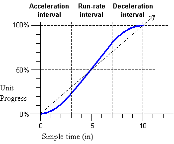
These attributes define a simple acceleration and deceleration of element time, within the simple duration. The values are expressed as a proportion of the simple duration (i.e. between 0 and 1), and are defined such that the length of the simple duration is not changed by the use of these attributes. The normal play speed within the simple duration is increased to compensate for the periods of acceleration and deceleration (this is how the simple duration is preserved). The modified speed is termed the run rate. As the simple duration progresses (i.e., plays back), acceleration causes the rate of progress to increase from a rate of 0 up to the run rate. Progress continues at the run rate until the deceleration phase, when progress slows from the run-rate down to a rate of 0. This is illustrated in Figure 1, below:
<animation dur="10s" accelerate="0.3" decelerate="0.3" .../>
Figure 1: Effect of acceleration and deceleration upon the rate of progress.
These attributes apply to the simple duration; if these attributes are combined with repeating behavior, the acceleration and/or deceleration occurs within each repeat iteration.
The sum of accelerate and decelerate must not exceed 1. If the individual values of the accelerate and decelerate attributes are between 0 and 1 and the sum is greater than 1, then both the accelerate and decelerate attributes will be ignored and the timed element will behave as if neither attribute was specified.
If the simple duration of the element is not resolved or if it is resolved to be indefinite, then the accelerate and decelerate attributes are ignored.
For details of computing the run-rate, and for converting from parent simple time to element simple time when accelerate and/or decelerate are specified, see Computing the element run-rate and Converting document time to element time.
In this example, a motion path will accelerate up from a standstill over the first 2 seconds, run at a faster than normal rate for 4 seconds, and then decelerate smoothly to a stop during the last 2 seconds. This makes the motion animation look more realistic.
<img ...>
    <animateMotion dur="8s" accelerate=".25" decelerate=".25" .../>
</img>
In the following example, the image will "fly in" from offscreen left, and then decelerate during the last second to "ease in" to place. This assumes a layout model that supports positioning (for example CSS positioning, or the position of a region in SMIL Layout).
<img ...>
    <animate attributeName="left" dur="4s" decelerate=".25"
             from="-1000" to="0" additive="sum" />
</img>
Another common mechanical phenomenon is that of a process that advances and reverses. Some examples include:
Because so many common use-cases apply repeat to the modified local time (as in the examples above), this function is modeled as modifying the simple duration. As such, autoReverse doubles the declared or implicit simple duration. When combined with repeating behavior, each repeat iteration will play once forwards, and once backwards.
When this is applied to a time container, it will play the time container forwards and then backwards. The semantics of playing a time container backwards are detailed in Implications of time manipulations on time containers.
The autoReverse time manipulation does not initially require a resolved simple duration, although it will not begin playing backwards until the simple duration is resolved and has completed. This can happen when the simple duration is defined by an unresolved implicit simple duration (such as the intrinsic media duration). In this case, the element will continue to play forward until the implicit simple duration is resolved (or until the active duration or the parent time container cuts short the simple duration, as described in the Timing section of SMIL 2.0). If the implicit simple duration becomes resolved before the end of the active duration, then the simple duration will be resolved to 2 times this implicit duration, and the implicit simple duration will play backwards.
Any time that the element will play backwards, including the second part of the autoReverse manipulation, the simple duration must be resolved. See also The speed attribute.
In this example, a motion path will animate normally for 5 seconds moving the element 20 pixels to the right, and then run backwards for 5 seconds (from 20 pixels to the right back to the original position). The repeating behavior causes it to repeat this 2 more times, finally leaving the element at its original location. The computed simple duration of the animation is 10 seconds, and the active duration is 30 seconds.
<img ...>
    <animateMotion by="20, 0" dur="5s" autoReverse="true" repeatCount="3"/>
</img>
In the following example the motion path will behave as above, but will end at the earlier of 15 seconds or when the user clicks on the image. If the element ends at 15 seconds (if the user does not click), the motion path will leave the element at the end of the defined path, 20 pixels to the right. Since the active duration is defined by the repeatDur and end, the active duration is not affected by the autoReverse attribute in this case. The semantics of fill are not changed by time manipulations: the media state at the end of the active duration is used during any fill period. The end of the active duration may fall part of the way through a play forward interval, or part of the way through a play backward interval.
<img ...>
    <animateMotion  by="20, 0" dur="5s" autoReverse="true"
         repeatDur="15" end="click" fill="freeze"/>
</img>
The accelerate and decelerate attributes can be combined with autoReverse, and are applied to the unmodified simple duration. For example:
<img ...>
    <animateMotion by="20, 0" dur="4s" autoReverse="true"
       accelerate=".25" decelerate=".25" />
</img>
This will produce a kind of elastic motion with the path accelerating for 1 second from the original position as it moves to the right, moving slightly faster than normal for 2 seconds, and then decelerating for 1 second as it nears the points 20 pixels to the right. It accelerates back towards the original position and decelerates to the end of the reversed motion path, at the original position.
The following example of a rotation (based upon the SVG animateTransform element) also demonstrates the combination of accelerate, decelerate and autoReverse. It will produce a simple pendulum swing on the target (assume that the target is a pendulum shape with the transform origin at the top):
<animateTransform type="rotate" from="20" to="-20" dur="1s" repeatCount="indefinite"
        accelerate=".5" decelerate=".5" autoReverse="true" ... />
The pendulum swings through an arc in one second, and then back again in a second. The acceleration and deceleration are applied to the unmodified simple duration, and autoReverse plays this modified simple duration forwards and then backwards. The effect is to accelerate all the way through the downswing, and then decelerate all through the upswing. The autoReverse feature then makes the same animation (i.e. the simple duration) play in reverse, and the pendulum swings back to the starting position. The entire modified simple duration repeats, producing continuous back and forth animation. This produces a realistic looking animation of real-world pendulum motion.
The speed attribute controls the local playback speed of an element, to speed up or slow down the effective rate of play relative to the parent time container. The speed attribute is supported on all timed elements. The argument value does not specify an absolute play speed, but rather is relative to the playback speed of the parent time container. The specified value cascades to all time descendents. Thus if a par and one of its children both specify a speed of 50%, the child will play at 25% of normal playback speed.
Values less than 0 are allowed, and cause the element to play backwards. An element can only play backwards if there is sufficient information about the simple and active durations. Specifically:
If the cascaded speed value for the element is negative and if either of the above two conditions is not met, the element will begin and immediately end (i.e. it will behave as though it had a specified active duration of 0). If there is a min attribute specified, the time container will simply be frozen at the initial state for the specified minimum duration.
The details of the effect of the element speed upon the timing calculations are described in Details of timing model arithmetic.
The following motion animation will move the target twice as fast as normal:
<animateMotion dur="10s" repeatCount="2" speed="2.0" path= ... />
The target will move over the path in 5 seconds (simple dur/speed =10s/2.0 = 5s), and then repeat this motion (because repeatCount is set to 2). The active duration is thus 10 seconds.
When speed is applied to a time container, it scales the rate of progress through the time container timeline. This effect cascades. When descendents also specify a speed value, the parent speed and the child speed are multiplied to yield the result. For example:
<par speed=2.0>
   <animate begin="2s" dur="9s" speed=0.75 .../>
</par>
The observed rate of play of the animate element is 1.5 times the normal play speed (2.0 * 0.75 == 1.5). The element begins 1 second after the par begins (the begin offset is scaled only by the parent speed), and ends 6 seconds later (dur/speed = 9/1.5 = 6).
The following example shows how an event based end combines with time manipulations:
<par speed=2.0>
   <animate begin="2s" dur="9s" speed=0.75
        repeatCount="4" end="click" .../>
</par>
This behaves as in the first example, but the animate element will repeat 4 times for an observed time of 24 seconds (dur/cascaded speed = 9s/(2.0 * 0.75) = 6s, and 6s * 4 repeats = 24s). If a click occurs before this, the element ends at the time of the click. A variant on this demonstrates syncbase timing:
<par speed=2.0>
   <img id="foo" dur="30s" .../>
   <animate dur="9s" speed=0.75
        repeatCount="4" end="click; foo.end" .../>
</par>
The image will display for 15 seconds. The animate element plays at an observed rate of 1.5 times play speed (2.0 * 0.75), but it will end after 15 seconds, when the image ends. The observed simple duration will be 6 seconds long (9 seconds divided by the cascaded speed 1.5). The animation will repeat 2.5 times during the active duration. Note that although the animation has a speed value, this does not impact the semantic of the syncbase timing. When the syncbase, eventbase, wallclock or media marker time is observed to happen, it will be applied anywhere it is used at that actual time (although conversions are applied internally, e.g. from syncbase element active time to parent simple time - see also Converting document time to element time).
Note that in the examples above, the default duration of the par container is defined as endsync="last". This behavior is not affected by the speed modifications, in the sense that the observed end of the elements will produce the correct simple duration on the parent time container.
The following example illustrates an important effect of offset time scaling:
<par speed=2.0>
   <img id="foo" dur="30s" .../>
   <animate begin="2s" dur="9s" speed=0.75
        repeatCount="4" end="foo.end+6s" .../>
</par>
The image will display for 15 seconds, as above. The animate element begins at 1 second, since the begin offset is scaled by the parent time container speed, but not by the element speed. The animate element will end at 18 seconds (15 seconds plus 6 seconds divided by the time container speed of 2.0). The "6s" offset added to "foo.end" is scaled by the parent time container speed, but not by the element speed.
This section is normative
When the time manipulation attributes are used to adjust the speed and/or pacing within the simple duration, the semantics can be thought of as changing the pace of time in the given interval. An equivalent model is these attributes simply change the pace at which the presentation progresses through the given interval. The two interpretations are equivalent mathematically, and the significant point is that the notion of "time" as defined for the element simple duration should not be construed as real world clock time. For the purposes of SMIL Time manipulations (as for SMIL Timing and Synchronization), "time" can behave quite differently from real world clock time.
In the following discussion, several symbols are used as shorthand:
Let a be the value of accelerate, and b be the value of decelerate. Both take on (floating point) values 0 to 1, and will not sum to more than 1.
Let dur be the value of the simple duration as defined by the Timing and Synchronization model. This is the actual simple duration, and not simply the dur attribute. This value does not account for the effect of any time manipulations.
Let dacc be the duration of the acceleration phase, and ddec be the duration of the deceleration phase. These values are computed as a function of the unmodified simple duration. Note that with the described model for acceleration and deceleration, the observed duration during which time accelerates and/or decelerates may be greater than dacc and ddec respectively.
dacc = dur * addec = dur * d
In order to preserve the simple duration, the speed through the simple duration must be increased to account for acceleration and deceleration. To compute the run rate over the course of the simple duration, the following formula is used. The run rate r is then:
r = 1 / ( 1 - a/2 - b/2 )
Thus, for example, if the value of accelerate is 1 (i.e. accelerate throughout the entire simple duration), the run rate is 2 (twice the normal play speed).
r(t) is the speed modification due to acceleration and deceleration, at any time t within the simple duration. The parameter time t must not already be modified to account for acceleration and deceleration. In the terms of the discussion below, Converting document time to element time, the parameter time t is in the tsu' space. The speed modification is defined as a function of the run rate r, as follows:
In the acceleration interval, where (0 <= t < dacc)r(t) = r * ( t / dacc )In the run-rate interval, where (
dacc <= t <= ( dur - ddec ))r(t) = rIn the deceleration interval, where (
( dur - ddec ) < t <= dur)r(t) = r * ( dur - t ) / ( ddec )
The run-rate only describes the modification applied to account for any acceleration and deceleration. This is combined with any element speed, as well as the speed inherited from the parent time container. The combined or "net" speed is defined in the section Computing the net cascaded speed for an element.
To convert a document time to an element time, the original time is converted to a simple time for each time container from the root time container down to the parent time container for the element. This recursive algorithm allows for a simple model of the conversion from parent simple time to element active and element simple time. The first step calculates element active time, and the second step calculates element simple time.
These steps are based upon a simpler, general model for time conversion that applies to the timing model independent of the time manipulations functionality (see also the Timing section of SMIL 2.0). The steps below describe the modified arithmetic for converting times, taking into account the semantics of time manipulations.
The steps below assume that the associated times are resolved and not indefinite. If a required time is not resolved or is indefinite, then the conversion is not defined, and cannot be performed.
In order to reflect the semantics of element speed, the element active time must be adjusted. The adjusted time is called the filtered active time, and is used by the element where the timing semantics refer to "element active time". The autoReverse and accelerate /decelerate attributes only affect the computation of the filtered simple time, and so do not come into play in this step.
The input time is a time in parent simple time. This is normalized to the element active duration, adjusting for the accumulated synchronization offset (described in The accumulated synchronization offset).
Let tps be a time in parent simple time, and B be the begin time, and O be the accumulated synchronization offset for an element, measured in parent simple time.The unfiltered active time tau for any child element is:
tau = tps - B - O
Given an unfiltered active tau, the filtered active time taf is only a function of the speed for the element (this is the value specified in a speed attribute, or the default, and not the net cascaded speed):
If( speed > 0 ) i.e. if the local speed is forwardstaf = tau * speedElse i.e. if the local speed is backwards
taf = AD - tau * ABS( speed )
As expected, if the speed value is 1 (the default), this is an identity function, and so taf = tau. When speed is less than 0 (in the backwards direction), the active duration proceeds from the end of the active duration towards 0.
In order to reflect the semantics of the autoReverse and accelerate /decelerate attributes, the element simple time must be adjusted. The adjusted time is called the filtered simple time. The filtered simple time is defined as a function of the filtered active time, and so reflects all the time manipulations on an element.
The element simple time is the time that is used to establish runtime synchronization for a media element, or to compute an animation function's input value or sampling time. If the element is a time container, this is also the time that is seen by all children of a time container (as the time container element's simple time).
The input time is a filtered active time taf.
Let dur' be the modified simple duration that accounts for the effect of the autoReverse attribute. It is computed as follows:If autoReverse is false:dur' = dur
Else (if autoReverse is true)
dur' = dur * 2
The steps to compute the filtered simple time are described below.
If there is no repeating behavior:
tsu = taf
Else, if the modified simple duration dur' is fixed and does not vary (ideal case):
tsu = REMAINDER( taf, dur' )
where REMAINDER( t, d ) is defined as (t - d*floor(t/d)).
Else, if the modified simple duration dur' varies from repeat iteration to repeat iteration, or if it is unknown, then the unfiltered simple time is just computed from the begin time of the most recent iteration - call this tlast-repeat. Some other mechanism (such as endsync logic or a media player) must note when the simple duration ends, and reset the value of tlast-repeat. If the element has not yet repeated, a value of 0 is used in place of tlast-repeat.
tsu = taf - tlast-repeat
Else if autoReverse is true (note that the following steps use the unmodified duration dur, and not dur'):
If tsu < durtsu' = tsuElse ( tsu >= dur )
tsu' = dur - ( tsu - dur ) = 2*dur - tsu
The filtered simple time tsf is computed as a function of the input time tsu' and the run rates in effect over the interval from 0 to tsu'. The filtered simple time is the accumulated progress up to the input time, and is computed as the integral of the acceleration, run-rate and deceleration rates. Since the rate of acceleration and deceleration are constant, the integral simplifies to a function of the average rate of progress for each of the three intervals defined by the acceleration and deceleration values. The steps below compute the filtered time by multiplying the input time and the average rates of progress. In the acceleration interval, since acceleration is constant and the rate changes from 0 to r, the average rate is just 1/2 of the instantaneous rate r(t) defined above:average rate = (r(t) + r(0) ) / 2) = r(t)/2In the deceleration interval, the average rate is similarly computed. In the run-rate interval the rate is constant, and so the average rate is equal to the run-rate.
In the acceleration interval, where ( 0 <= tsu' < dacc ), the filtered simple time is the input time multiplied by the average run-rate during the acceleration interval:
tsf = tsu' * r(tsu') / 2In the run-rate interval, where ( dacc <= tsu' <= ( dur - ddec ) ), the filtered simple time is computed from the input time and the rates in the acceleration and run-rate intervals. This adds the accumulated progress in the acceleration interval to the progress within the run-rate interval:
tsf = dacc * r / 2 + ( tsu' - dacc ) * r= r * ( dacc / 2 + ( tsu' - dacc ))
= r * ( tsu' - dacc / 2 )
In the deceleration interval, where ( ( dur - ddec ) < tsu' <= dur ), the filtered simple time is computed from the input time and the rates in all three intervals. This sums the total progress in the acceleration interval, the total progress within the run-rate interval, and the progress within the deceleration interval.
To simplify the expressions, we define tdec, the time spent in the deceleration interval:
tdec = tsu' - ( dur - ddec )We also define the proportional duration within the deceleration interval as:
pd = tdec / ddecThe filtered time within the deceleration interval is then:
tsf = dacc * r / 2
+ ( dur - dacc - ddec ) * r
+ tdec * (( r + r*(1 - pd )) / 2 ))= r * ( dur - dacc / 2 - ddec
+ tdec * ( 2 - pd ) / 2 )
To convert from one element timespace to another, the time for the first element te1 must first be converted to a simple time on the closest ascendant time container that contains both elements. Converting from an element time to the parent time reverses the process described above. Again, it is recursive, and so the conversions are described generically from element simple to element active time, and from element active to parent simple time.
To convert from element simple time to element active time requires the begin time of the most recent iteration, tlast-repeat. If the element does not repeat or has not yet repeated, a value of 0 is used in place of tlast-repeat.
ta = ts + tlast-repeat
Conversion from element active time to parent simple time uses the associated begin of the element and the accumulated synchronization offset.
tps = ta + B + O
Note that the pure conversions do not take into account the clamping of active durations, nor the effects of fill (where time is frozen). Global to local time conversions used to translate between timespaces must ignore these issues, and so may yield a time in the destination local timespace that is well before or well after the simple duration of the element.
An alternate form of the conversion is used when actually sampling the time graph. A time container is only sampled if it is active or frozen, and so no times will be produced that are before a time container begins. If the global to local time conversion for a time container yields a time during which the time container is frozen, the time is clamped to the value of the active end.
The net cascaded speed for a given element at a given point in time can be used to set the correct playback rate for a media element. It is not otherwise used directly in the time manipulations model.
To compute the net cascaded speed speednc(t) for an element at a given point in time, we combine the net cascaded parent speed at the point in time speednc-parent(t) with the element speed value speed and the instantaneous run rate r(t) computed from any acceleration and deceleration. If the element has no time parent, use 1 for speednc-parent(t).
Note that the net cascaded parent speed will be computed in simple time for the parent, and so the element simple time will have to be converted to a parent simple time. This is described above in Converting element time to document time.
The parameter time value must be in the range of the simple duration. The time value must not already be modified to account for acceleration and deceleration. In the terms of the discussion above, Converting document time to element time, the parameter time is in the tsu' space.
The net cascaded speed speednc(t) for a given unfiltered simple time tsu' is then:
speednc(tsu') = speednc-parent(tsu') * speed * r(tsu')
This definition is recursive up to the root of the time containment hierarchy, and so accounts for any speed settings on the parent and all other ascendant time containers.
This section is informative
A theoretical model can be described that assumes that all element local timelines (including any media elements) are completely non-linear and have unconstrained ballistics (i.e. they can be sampled at any point at any moment, and can adjust the observed playback rate instantaneously). This ideal model can be applied to many applications, including pure rendered graphics, text, etc. Nevertheless, many common applications also include media with linear behavior and other limitations on playback. When the timegraph includes media elements that have linear behavior, the time manipulations model must accommodate these real world limitations.
While the model does support timegraphs with a mix of linear and non-linear behavior, and defines specific semantics for media elements that cannot support the ideal non-linear model, it is not a goal to provide an ideal alternative presentation for all possible timegraphs with such a mix. It is left to authors and authoring tools to apply the time manipulations in appropriate situations. This section describes both the ideal model as well as the semantics associated with linear-media elements.
This section is informative
In the ideal model, the pace or speed of local time can be manipulated arbitrarily. The graph advances (or is sampled, depending upon your perspective) as the presentation time advances. A time container samples each of its children in turn, so that a graph traversal is performed for each render time. Elements that are neither active nor frozen may be pruned from the traversal as an optimization. As the traversal moves down the graph (from time containers to children), each local timeline simply transforms the current time from the parent time-space to the local time space, and then samples the local timeline at the transformed current time. Note that the speed and effects of the time filters effectively cascade down the time graph, since each element transforms element time and element speed for itself and all descendents.
This is the model that is described by the arithmetic model in Details of timing model arithmetic.
When linear media are added to this model and the "current time" (sample) traversal encounters a media element, the media element is effectively told to "sample" at a particular position and a particular rate. Given that linear media can not sample arbitrarily (i.e., they cannot immediately seek to and display an arbitrary frame or sample) , the media element player may not be able to match the ideal model.
Many media elements cannot play off-speed (i.e. at other than normal play
speed), and so must simply ignore the requested speed. As the element plays,
it will fall out of sync with the sync relationship defined in the timing
syntax. Within the limits defined by the SMIL syncTolerance attribute,
divergence from the theoretical timeline position may be ignored. However,
for further divergence beyond this tolerance the element will be considered
out of sync; if the element is defined with
syncBehavior="locked", the playback engine will try to enforce
the runtime synchronization semantics (and this will probably not yield a
desirable presentation playback). Authors applying time manipulations to
linear media or to time containers that include linear media will likely wish
to specify the syncBehavior for the linear
media as "canSlip".
This section is normative
The fallback semantics depend upon how much or how little the media player is capable of. Some players for some media may play forwards and backwards but only at the normal rate of play, others may only support normal forward play speed.
If the element speed (i.e. the cascaded value) is not supported by the media element, the media should play at the closest supported speed ("best effort"). If the element cannot play slower or faster than the normal play speed, the closest supported speed will be the normal play speed.
In any case, the computed simple duration, as modified by the time filters, is respected.
The semantics of clipBegin and clipEnd are not affected by time manipulations. The clipBegin and clipEnd semantics are always interpreted in terms of normal forward play speed. They are evaluated before any effects of time filters have been applied to the time model. This is consistent with the model that they can be evaluated by the media element handler, independent of the time model.
This section is informative
In this fallback model, some media elements may not be able to play at the computed speed defined by the time graph. The fallback semantics may cause the media element to fall out of visual synchronization with respect to the rest of the timegraph. For example, if an image element is defined to begin 10 seconds after a video element begins, and then a speed of 2.0 is applied to a time container for both elements, the image element will begin at 5 seconds (10s/2.0). If the video cannot play at twice the normal speed, it will not be 10 seconds into the video when the image shows up, and so the presentation may appear to be out of sync.
When time manipulations are used with linear media, authors can use media-marker-values to define the sync relationships. This can help to maintain the "visual" sync regardless of the fallback behavior. Since the media-marker-values are defined to happen when a particular point in the media is played, this timing will respect the actual behavior of the media, rather than the computed speed behavior.
This section is normative
The time manipulations can apply to any element, including time containers. There are two primary implications of this for the time model:
The following discussion is based upon the semantics of begin and end instance lists and the interpretation of lists of begin and end times described in the Timing section of SMIL 2.0
If the time container can play backwards (based upon the general constraints for backwards play upon the simple and active durations), then the children must play the defined intervals in reverse order. This is accomplished with the following modified life cycle for child elements. In the following description, the terms "begin" and "end" for intervals are used relative to the normal play direction. When used as a verb ("the interval begins"), begin and end refer to the current interval becoming active and inactive, respectively. Intervals are described as playing from the end of the interval to the beginning, and so they begin at the interval end, and end at the interval begin.
When a time container is defined to play backwards, a child element may define additional time manipulations that affect the speed, or even the direction of play. Any such additional time manipulations on the child element do not impact the model described above.
The life cycle is restarted each time the parent (or any ascendant) time container repeats or restarts, just as for the normal play direction.
Because of the reversed evaluation of intervals, some cyclic time dependencies that would correctly propagate forwards when played normally will not propagate correctly when played backwards. The rules for evaluating and halting cycles in the time graph are unchanged by the semantics of time manipulations.