A model for adding declarative raster-based rendering effects to a 2D graphics environment is presented. As a result, the expressiveness of the traditional 2D rendering model is greatly enhanced, while still preserving the device independence, scalability, and high level geometric description of the underlying graphics.
On the Web, many graphics are presented as bitmap images in gif, jpg, or png format. Among the many disadvantages of this approach is the general difficulty of keeping the raster data in sync with the rest of the Web site. Many times, a web site designer must resort to a bitmap editor to simply change the title of a button. As the Web gets more dynamic, we desire a way to describe the "piece parts" of a site in a more flexible format. This chapter describes SVG's declarative filter effects model, which when combined with the 2D power of SVG can describe much of the common artwork on the web in such a way that client-side generation and alteration can be performed easily.
The filter effects model consists of a set of filtering operations (called "processing nodes" in the descriptions below) on one or more graphic primitives. Each processing node takes a set of graphics primitives as input, performs some processing, and generates revised graphics primitives as output. Because nearly all of the filtering operations are some form of image processing, in almost all cases the output from most processing nodes consists of a single RGBA image.
For example, a simple filter could replace one graphic by two -- by adding a black copy of original offset to create a drop shadow. In effect, there are now two layers of graphics, both with the same original set of graphics primitives. In this example, the bottommost shadow layer could be blurred and become a raster layer, while the topmost layer could remain as higher-order graphics primitives (e.g., text or vector objects). Ultimately, the two layers are composited together and rendered into the background.
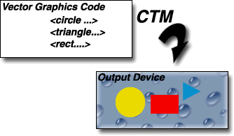
Filter effects introduce an additional step into the traditional 2D graphics pipeline. Consider the traditional 2D graphics pipeline:
Vector graphics primitives are specified abstractly and rendered onto the output device through a geometric transformation called the current transformation matrix, or CTM. The CTM allows the vector graphics code to be specified in a device independent coordinate system. At rendering time, the CTM accounts for any differences in resolution or orientation of the input vector description space and the device coordinate system. According to the "painter's model", areas on the device which are outside of the vector graphic shapes remain unchanged from their previous contents (in this case the droplet pattern).
Consider now, altering this pipeline slightly to allow rendering the graphics to an intermediate continuous tone image which is then rendered onto the output device in a second pass:
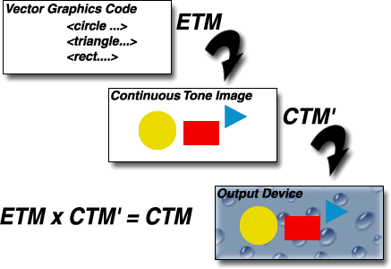
We introduce a new transformation matrix called the Effect Transformation Matrix, or ETM. Vector primitives are rendered via the ETM onto an intermediate continuous tone image. This image is then rendered onto the output device using the standard 2D imaging path via a modified transform, CTM', such that the net effect of ETM followed by CTM' is equivalent to the original CTM. It is important to note that the intermediate continuous tone image contains coverage information so that non rendered parts of the original graphic are transparent in the intermediate image and remain unaffected on the output device, as required by the painter's model. A physical analog to this process is to imagine rendering the vector primitives onto a sheet of clear acetate and then transforming and overlaying the acetate sheet onto the output device. The resulting imaging model remains as device-independent as the original one, except we are now using the 2D imaging model itself to generate images to render.
So far, we really haven't added any new expressiveness to the imaging model. What we have done is reformulated the traditional 2D rendering model to allow an intermediate continuous tone rasterization phase. However, now we can extend this further by allowing the application of image processing operations on the intermediate image, still without sacrificing device independence. In our model, the intermediate image can be operated on by a number of image processing operations which can effect both the color and coverage channels. The resulting image(s) are then rendered onto the device in the same way as above.
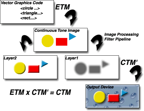
In the picture above, the intermediate set of graphics primitives was processed in two ways. First a simple bump map lighting calculation was applied to add a 3D look, then another copy of the original layer was offset, blurred and colored black to form a shadow. The resulting transparent layers were then rendered via the painter's model onto the output device.
Filter effects are defined by a <filter> element with an associated ID. Filter effects are applied to elements which have a filter: property which reference a <filter> element. Here is an example:
<?xml version="1.0" standalone="no"?>
<!DOCTYPE svg PUBLIC "-//W3C//DTD SVG July 1999//EN"
  "http://www.w3.org/Graphics/SVG/svg-19990730.dtd">
<svg width="4in" height="3in">
  <defs>
    <filter id="CoolTextEffect">
      <!-- Definition of filter goes here -->
    </filter>
  </defs>
  <text style="filter:url(#CoolTextEffect)">Text with a cool effect</text>
</svg>
When applied to grouping elements such as <g>, the filter: property applies to the contents of the group as a whole. The effect should be as if the group's children did not render to the screen directly but instead just added their resulting graphics primitives to the group's graphics display list (GDL), which is then passed to the filter for processing. After the group filter is processed, then the result of the filter should be rendered to the target device (or passed onto a parent grouping element for further processing in cases such as when the parent has its own group filter).
The <filter> element consists of a sequence of processing nodes which take a set of graphics primitives as input, apply filter effects operations on the graphics primitives, and produce a modified set of graphics primitives as output. The processing nodes are executed in sequential order. The resulting set of graphics primitives from the final processing node (feMerge in the example below) represents the result of the filter. Here is an example:
<?xml version="1.0" standalone="no"?>
<!DOCTYPE svg PUBLIC "-//W3C//DTD SVG July 1999//EN"
  "http://www.w3.org/Graphics/SVG/svg-19990730.dtd">
  <filter id="Shadow">
    <feGaussianBlur     in="SourceAlpha"
                        radius="3"
                        nodeId="blurredAlpha" />
    <feOffset           in="blurredAlpha"
                        dx="2" dy="1"
                        nodeId="offsetBlurredAlpha" />
    <feDiffuseLighting  in="blurredAlpha"
                        diffuseConstant=".5"
                        nodeId="bumpMapDiffuse" >
      <feDistantLight/>
    </feDiffuseLighting>
    <feComposite        in="bumpMapDiffuse" in2="SourcePaint"
                        operator="arithmetic" k1="1"
                        nodeId="litPaint" />
    <feSpecularLighting in="blurredAlpha"
                        specularConstant=".5"
                        specularExponent="10"
                        lightColor="feDistantLight"
                        nodeId="bumpMapSpecular" >
      <feDistantLight/>
    </feSpecularLighting>
    <feComposite        in="litPaint" in2="bumpMapSpecular"
                        operator="arithmetic" k2="1" k3="1"
                        nodeId="litPaint" />
    <feComposite        in="litPaint"
                        in2="SourceAlpha"
                        mode="AinB"
                        nodeId="litPaint" />
    <feMerge>
      <feMergeNode in="litPaint" />
      <feMergeNode in="offsetBlurredAlpha" />
    </feMerge>
  </filter>

  <text style="font-size:36; fill:red; filter:url(#Shadow)"
        x="10" y="250">Shadowed Text</text>
</svg>
For most processing nodes, the in (and sometimes in2) attribute identifies the graphics which serve as input and the nodeId attribute gives a name for the resulting output. The in and in2 attributes can point to either:
The default value for in is the output generated from the previous processing node. In those cases where the output from a given processing node is used as input only by the next processing node, it is not necessary to specify the nodeId on the previous processing node or the in attribute on the next processing node. In the example above, there are a few cases (show highlighted) where nodeId and in did not have to be provided.
Filters do not use XML IDs for nodeIds; instead, nodeIds can be any arbitrary attribute string value. nodeIds only are meaningful within a given <filter> element and thus have only local scope. If a nodeId appears multiple times within a given <filter> element, then a reference to that nodeId will use the closest preceding processing node with the given nodeId. Forward references to nodeIds are invalid.
A <filter> element can define a region on the canvas on which a given filter effect applies and can provide a resolution for any intermediate continuous tone images used in to process any raster-based processing nodes. The <filter> element has the following attributes:
x-pixels [y-pixels])
and indicates
the width/height of the intermediate images in pixels. If not provided,
then a reasonable default resolution appropriate for the target device
will be used. (For displays, an appropriate display resolution,
preferably the current display's pixel resolution, should be the default.
For printing, an appropriate
common printer resolution, such as 400dpi, should be the default.)For performance reasons on display devices, it is recommended that the filter effect region is designed to match pixel-for-pixel with the background.
It is often necessary to provide padding space because the filter effect might impact bits slightly outside the tight-fitting bounding box on a given object. For these purposes, it is possible to provide negative percentage values for x, y and percentages values greater than 100% for width, height. For example, x="-10%" y="-10%" width="110%" height="110%".
The following two attributes are available for all processing nodes (the exception is feMerge and feImage, which do not have an in attribute):
|
Common Attributes |
nodeId Assigned name for this node. If supplied, then the GDL resulting after processing the given node is saved away and can be referenced as input to a subsequent processing node. in If supplied, then indicates that this processing node should use either the output of previous node as input or use some standard keyword to specify alternate input. (For the first processing node, the default in is SourceGraphic.) Available keywords representing pseudo image inputs include:
|
Two possible pseudo input images for filter effects are BackgroundImage and BackgroundAlpha, which each represent an image snapshot of the canvas under the filter region at the time that the <filter> element is invoked. BackgroundImage represents both the color values and alpha channel of the canvas (i.e., RGBA pixel values), whereas BackgroundAlpha represents only the alpha channel.
Implementations of SVG user agents often will need to maintain supplemental background image buffers in order to support the BackgroundImage and BackgroundAlpha pseudo input images. Sometimes, the background image buffers will contain an in-memory copy of the accumulated painting operations on the current canvas.
Because in-memory image buffers can take up significant system resources, SVG documents must explicitly indicate to the SVG user agent that the document needs access to the background image before BackgroundImage and BackgroundAlpha pseudo input images can be used. The property which enables access to the background image is 'enable-background':
| Value: | accumulate | new [ ( <x> <y> <width> <height> ] ) |
| Initial: | accumulate |
| Applies to: | container elements |
| Inherited: | no |
| Percentages: | N/A |
| Media: | visual |
'enable-background' is only applicable to container elements and specifies how the SVG user agents should manage the accumulation of the background image.
A value of new indicates two things:
A meaning of enable-background: accumulate (the initial/default value) depends on context:
If a filter effect specifies either the BackgroundImage or the BackgroundAlpha pseudo input images and no ancestor container element has a property value of 'enable-background:new', then the background image request is technically in error. Processing should proceed without interruption (i.e., no error message) and a fully transparent image should be provided in response to the request.
The optional (<x>,<y>,<width>,<height>) parameters on the new value indicate the sub-region of user space where access to the background image is allowed to happen. These parameters enable the SVG user agent potentially to allocate smaller temporary image buffers than the default values, which might require the SVG user agent to allocate buffers as large as the current viewport. Thus, the values <x>,<y>,<width>,<height> act as a clipping rectangle on the background image canvas.
The following is a catalog of the individual processing nodes. Unless otherwise stated, all image filters operate on linear premultiplied RGBA samples. Filters which work more naturally on non premultiplied data (feColorMatrix and feComponentTransfer) will temporarily undo and redo premultiplication as specified. All raster effect filtering operations take 1 to N input RGBA images, additional attributes as parameters, and produce a single output RGBA image.
|
NodeType |
feBlend | ||||||||||||
|
Processing Node-Specific Attributes |
mode, One of the image blending modes (see table below). Default is: normal in2, The second image ("B" in the formulas) for the compositing operation. | ||||||||||||
|
Description |
This filter composites two objects together using commonly used high-end imaging software blending modes. Performs the combination of the two input images pixel-wise in image space. | ||||||||||||
|
Implementation Notes |
The compositing formula, expressed using premultiplied colors: qr = 1 - (1-qa)*(1-qb) cr = (1-qa)*cb + (1-qb)*ca + qa*qb*(Blend(ca/qa,cb/qb)) where: qr = Result opacity cr = Result color (RGB) - premultiplied qa = Opacity value at a given pixel for image A qb = Opacity value at a given pixel for image B ca = Color (RGB) at a given pixel for image A - premultiplied cb = Color (RGB) at a given pixel for image B - premultiplied Blend = Image compositing function, depending on the compositing mode The following table provides the list of available image blending modes:
|
|
NodeType |
feColor |
|
Processing Node-Specific Attributes |
color, RGBA color (floating point?) |
|
Description |
Creates an image with infinite extent filled with color |
|
NodeType |
feColorMatrix |
|
Processing Node-Specific Attributes |
type, string (one of: matrix, saturate, hue-rotate, luminance-to-alpha) values
|
|
Description |
This filter performs | R' | | a00 a01 a02 a03 a04 | | R | | G' | | a10 a11 a12 a13 a14 | | G | | B' | = | a20 a21 a22 a23 a24 | * | B | | A' | | a30 a31 a32 a33 a34 | | A | | 1 | | 0 0 0 0 1 | | 1 | for every pixel. The RGBA and R'G'B'A' values are automatically non-premultiplied temporarily for this operation. The following shortcut definitions are provide for compactness. The following tables show the mapping from the shorthand form to the corresponding longhand (i.e., matrix with 20 values) form:
saturate value (0..100)

   s = value/100

   | R' |     |0.213+0.787s  0.715-0.715s  0.072-0.072s 0  0 |   | R |

   | G' |     |0.213-0.213s  0.715+0.285s  0.072-0.072s 0  0 |   | G |

   | B' |  =  |0.213-0.213s  0.715-0.715s  0.072+0.928s 0  0 | * | B |

   | A' |     |           0            0             0  1  0 |   | A |

   | 1  |     |           0            0             0  0  1 |   | 1 |

hue-rotate value (0..360)

   | R' |     | a00  a01  a02  0  0 |   | R |

   | G' |     | a10  a11  a12  0  0 |   | G |

   | B' |  =  | a20  a21  a22  0  0 | * | B |

   | A' |     | 0    0    0    1  0 |   | A |

   | 1  |     | 0    0    0    0  1 |   | 1 |

   where the terms a00, a01, etc. are calculated as follows:

      | a11 a12 a13 |    [+0.213 +0.715 +0.072]
      | a21 a22 a13 | =  [+0.213 +0.715 +0.072] +
      | a11 a12 a13 |    [+0.213 +0.715 +0.072]

                                  [+0.787 -0.715 -0.072]
          cos(hue-rotate value) * [-0.212 +0.285 -0.072] +
                                  [-0.213 -0.715 +0.928]

                                  [-0.213 -0.715+0.928]
          sin(hue-rotate value) * [+0.143 +0.140-0.283]
                                  [-0.787 +0.715+0.072]

   Thus, the upper left term of the hue matrix turns out to be:

         .213 + cos(hue-rotate value)*.787 - sin(hue-rotate value)*.213


luminance-to-alpha

   | R' |     |      0        0        0  0  0 |   | R |

   | G' |     |      0        0        0  0  0 |   | G |

   | B' |  =  |      0        0        0  0  0 | * | B |

   | A' |     |  0.299    0.587    0.114  0  0 |   | A |

   | 1  |     |      0        0        0  0  1 |   | 1 |
|
|
Implementation issues |
These matrices often perform an identity mapping in the alpha channel. If that is the case, an implementation can avoid the costly undoing & redoing of the premultiplication for all pixels with A = 1. |
|
NodeType |
feComponentTransfer |
|
Processing Node-Specific Attributes | None. |
|
Processing Node-Specific Sub-Elements |
|
|
Description |
This filter performs component-wise remapping of data as follows: R' = feFuncR( R ) G' = feFuncG( G ) B' = feFuncB( B ) A' = feFuncA( A ) for every pixel. The RGBA and R'G'B'A' values are automatically non-premultiplied temporarily for this operation. When type="table", the transfer function consists of a linearly interpolated lookup table. k/N <= C < (k+1)/N => C' = vk + (C - k/N)*N * (vk+1 - vk) When type="linear", the transfer function consists of a linear function describes by the following equation: C' = slope*C + offset When type="gamma", the transfer function consists of the following equation: C' = amplitude*pow(C, exponent) + offset |
|
Comments |
This filter allows operations like brightness adjustment, contrast adjustment, color balance or thresholding. We might want to consider some predefined transfer functions such as identity, gamma, sRGB transfer, sine-wave, etc. |
|
Implementation issues |
Similar to the feColorMatrix filter, the undoing and redoing of the premultiplication can be avoided if feFuncA is the identity transform and A = 1. |
|
NodeType |
feComposite |
|
Processing Node-Specific Attributes |
operator, one of (over, in, out, atop, xor, arithmetic). Default is: over. arithmetic-constants, k1,k2,k3,k4 in2, The second image ("B" in the formulas) for the compositing operation. |
|
Description |
This filter performs the combination of the two input images pixel-wise in image space. over, in, atop, out, xor use the Porter-Duff compositing operations. For these operations, the extent of the resulting image can be affected. In other words, even if two images do not overlap in image space, the extent for over will essentially include the union of the extents of the two input images. arithmetic evaluates k1*i1*i2 + k2*i1 + k3*i2 + k4, using componentwise arithmetic with the result clamped between [0..1]. |
|
Comments |
arithmetic are useful for combining the output from the feDiffuseLighting and feSpecularLighting filters with texture data. arithmetic is also useful for implementing dissolve. |
|
NodeType |
feDiffuseLighting |
|
Processing Node-Specific Attributes |
resultScale (Multiplicative scale for the result.
This allows the result of the feDiffuseLighting nodeto represent
values greater than 1) |
|
Processing Node-Specific Sub-Elements |
|
|
Description |
Light an image using the alpha channel as a bump map. The resulting image is an RGBA opaque image based on the light color with alpha = 1.0 everywhere. The lighting caculation follows the standard diffuse component of the Phong lighting model. The resulting image depends on the light color, light position and surface geometry of the input bump map. Color or texture is mean to be applied via a multiply (mul) composite operation. Dr = (kd * N.L * Lr) / resultScale Dg = (kd * N.L * Lg) / resultScale Db = (kd * N.L * Lb) / resultScale Da = 1.0 / resultScale where kd = diffuse lighting constant N is a function of x and y and depends on the surface gradient as follows: The surface described by the input alpha image Ain (x,y) is: Z (x,y) = surfaceScale * Ain (x,y) Surface normal is calculated using the Sobel gradient 3x3 filter: Nx (x,y)= - surfaceScale * 1/4*(( I(x+1,y-1) + 2*I(x+1,y)
+ I(x+1,y+1))
- (I(x-1,y-1) + 2*I(x-1,y)
+ I(x-1,y+1)))
Ny (x,y)= - surfaceScale * 1/4*(( I(x-1,y+1) + 2*I(x,y+1) + I(x+1,y+1))
- (I(x-1,y-1) + 2*I(x,y-1)
+ I(x+1,y-1)))
Nz (x,y) = 1.0
N = (Nx, Ny, Nz) / Norm((Nx,Ny,Nz))
L, the unit vector from the image sample to the light is calculated as follows: For Infinite light sources it is constant: Lx = cos(azimuth)*cos(elevation) Ly = -sin(azimuth)*cos(elevation) Lz = sin(elevation) For Point and spot lights it is a function of position: Lx = Lightx - x Ly = Lighty - y Lz = Lightz - Z(x,y) L = (Lx, Ly, Lz) / Norm(Lx, Ly, Lz) where Lightx, Lighty, and Lightz are the input light position. Lr,Lg,Lb, the light color vector is a function of position in the spot light case only: Lr = Lightr*pow((-L.S),specularExponent) Lg = Lightg*pow((-L.S),specularExponent) Lb = Lightb*pow((-L.S),specularExponent) where S is the unit vector pointing from the light to the point (pointsAtX, pointsAtY, pointsAtZ) in the x-y plane: Sx = pointsAtX - Lightx Sy = pointsAtY - Lighty Sz = pointsAtZ - Lightz S = (Sx, Sy, Sz) / Norm(Sx, Sy, Sz) If L.S is positive no light is present. (Lr = Lg = Lb = 0) |
|
Comments |
This filter produces a light map, which can be combined with a texture image using the multiply term of the arithmetic <Composite> compositing method. Multiple light sources can be simulated by adding several of these light maps together before applying it to the texture image. |
|
NodeType |
feDisplacementMap |
|
Processing Node-Specific Attributes |
scale |
|
Description |
Uses Input2 to spatially displace Input1, (similar to the Photoshop displacement filter). This is the transformation to be performed: P'(x,y) <- P( x + scale * ((XC(x,y) - .5), y + scale * (YC(x,y) - .5)) where P(x,y) is the source image, Input1, and P'(x,y) is the destination. XC(x,y) and YC(x,y) are the component values of the designated by the xChannelSelector and yChannelSelector. For example, to use the R component of Image2 to control displacement in x and the G component of Image2 to control displacement in y, set xChannelSelector to "R" and yChannelSelector to "G". |
|
Comments |
The displacement map defines the inverse of the mapping performed. |
|
Implementation issues |
This filter can have arbitrary non-localized effect on the input which might require substantial buffering in the processing pipeline. However with this formulation, any intermediate buffering needs can be determined by scale which represents the maximum displacement in either x or y. |
|
NodeType |
feGaussianBlur |
|
Processing Node-Specific Attributes |
stdDeviation. |
|
Description |
Perform gaussian blur on the input image. The Gaussian blur kernel is an appoximation of the normalized convolution: H(x) = exp(-x2/ (2s2)) / sqrt(2* pi*s2) where 's' is the standard deviation specified by stdDeviation. This can be implemented as a separable convolution. For larger values of 's' (s >= 2.0), an approximation can be used: Three successive box-blurs build a piece-wise quadratic convolution kernel, which approximates the gaussian kernel to within roughly 3%. let d = floor(s * 3*sqrt(2*pi)/4 + 0.5) ... if d is odd, use three box-blurs of size 'd', centered on the output pixel. ... if d is even, two box-blurs of size 'd' (the first one centered one pixel to the left, the second one centered one pixel to the right of the output pixel one box blur of size 'd+1' centered on the output pixel. |
|
Implementation Issues |
Frequently this operation will take place on alpha-only images, such as that produced by the built-in input, SourceAlpha. The implementation may notice this and optimize the single channel case. If the input has infinite extent and is constant, this operation has no effect. If the input has infinite extent and is a tile, the filter is evaluated with periodic boundary conditions. |
|
NodeType |
feImage |
|
Processing Node-Specific Attributes |
href, reference to external image data. |
|
Description |
Refers to an external image which is loaded or rendered into an RGBA raster. If imaging-matrix is not specified, the image takes on its natural width and height and is positioned at 0,0 in image space. The imageref could refer to an external image, or just be a reference to another piece of SVG. This node produces an image similar to the builtin image source SourceGraphic except from an external source. |
|
NodeType |
feMerge |
|
Processing Node-Specific Attributes |
none |
|
Processing Node-Specific Sub-Elements | Each <feMerge> element can have any number of <feMergeNode> subelements, each of which has an in attribute. |
|
Description |
Composites input image layers on top of each other using the over operator with Input1 on the bottom and the last specified input, InputN, on top. |
|
Comments |
Many effects produce a number of intermediate layers in order to create the final output image. This filter allows us to collapse those into a single image. Although this could be done by using n-1 Composite-filters, it is more convenient to have this common operation available in this form, and offers the implementation some additional flexibility (see below). |
|
Implementation issues |
The canonical implementation of feMerge is to render the entire effect into one RGBA layer, and then render the resulting layer on the output device. In certain cases (in particular if the output device itself is a continuous tone device), and since merging is associative, it may be a sufficient approximation to evaluate the effect one layer at a time and render each layer individually onto the output device bottom to top. |
|
NodeType |
feMorphology |
|
Processing Node-Specific Attributes |
operator,one of erode or dilate. |
|
Description |
This filter is intended to have a similar effect as the min/max filter in Photoshop and the width layer attribute in ImageStyler. It is useful for "fattening" or "thinning" an alpha channel, The dilation (or erosion) kernel is a square of side 2*radius + 1. |
|
Implementation issues |
Frequently this operation will take place on alpha-only images, such as that produced by the built-in input, SourceAlpha. In that case, the implementation might want to optimize the single channel case. If the input has infinite extent and is constant, this operation has no effect. If the input has infinite extent and is a tile, the filter is evaluated with periodic boundary conditions. |
|
NodeType |
feOffset |
|
Processing Node-Specific Attributes |
dx,dy |
|
Description |
Offsets an image relative to its current position in the image space by the specified vector. |
|
Comments |
This is important for effects like drop shadow etc. |
|
NodeType |
feSpecularLighting |
|
Processing Node-Specific Attributes |
surfaceScale height of surface when Ain = 1. specularConstant ks in Phong lighting model. Range 0.0 to 1.0 specularExponent exponent for specular term, larger is more "shiny". Range 1.0 to 128.0. lightColor RGB |
|
Processing Node-Specific Sub-Elements |
|
|
Description |
Light an image using the alpha channel as a bump map. The resulting image is an RGBA image based on the light color. The lighting caculation follows the standard specular component of the Phong lighting model. The resulting image depends on the light color, light position and surface geometry of the input bump map. The result of the lighting calculation is added. We assume that the viewer is at infinity the z direction (i.e the unit vector in the eye direction is (0,0,1) everywhere. Sr = ks * pow(N.H, specularExponent) * Lr Sg = ks * pow(N.H, specularExponent) * Lg Sb = ks * pow(N.H, specularExponent) * Lb Sa = max(Sr, Sg, Sb) where ks = specular lighting constant N = surface normal unit vector, a function of x and y H = "halfway" unit vectorbetween eye unit vector and light unit vector Lr,Lg,Lb = RGB components of light See feDiffuseLighting for definition of N and (Lr, Lg, Lb). The definition of H reflects our assumption of the constant eye vector E = (0,0,1): H = (L + E) / Norm(L+E) where L is the light unit vector. Unlike the feDiffuseLighting, the feSpecularLighting filter produces a non-opaque image. This is due to the fact that specular result (Sr,Sg,Sb,Sa) is meant to be added to the textured image. The alpha channel of the result is the max of the color components, so that where the specular light is zero, no additional coverage is added to the image and a fully white highlight will add opacity. |
|
Comments |
This filter produces an image which contains the specular reflection part of the lighting calculation. Such a map is intended to be combined with a texture using the add term of the arithmetic Composite method. Multiple light sources can be simulated by adding several of these light maps before applying it to the texture image. |
|
Implementation issues |
The feDiffuseLighting and feSpecularLighting filters will often be applied together. An implementation may detect this and calculate both maps in one pass, instead of two. |
|
NodeType |
feTile |
|
Processing Node-Specific Attributes |
none |
|
Description |
Creates an image with infinite extent by replicating source image in image space. |
|
NodeType |
feTurbulence |
|
Processing Node-Specific Attributes |
baseFrequency |
|
Description |
Adds noise to an image using the Perlin turbulence-function. It is possible to create bandwidth-limited noise by synthesizing only one octave. For a detailed description the of the Perlin turbulence-function, see "Texturing and Modeling", Ebert et al, AP Professional, 1994. If the input image is infinite in extent, as is the case with a constant color or a tile, the resulting image will have maximal size in image space. |
|
Comments |
This filter allows the synthesis of artificial textures like clouds or marble. |
|
Implementation issues |
It might be useful to provide an actual implementation for the turbulence function, so that consistent results are achievable. |